What is the Purpose of the IFERROR Function in Excel?

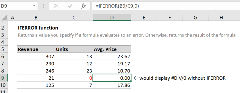
The IFERROR function in Excel is a powerful tool that allows you to handle errors and display custom messages or values. In this step-by-step guide, we’ll explore the purpose and usage of the IFERROR function.

Step 1: Identify the formula with potential errors

Look for formulas in your Excel worksheet that may generate errors, such as #DIV/0!, #N/A, #VALUE!, etc. It’s important to identify these formulas before applying the IFERROR function.

Step 2: Select the cell to contain the IFERROR formula

Choose the cell where you want the result or custom message to appear.

Step 3: Use the IFERROR function

Start the formula with “=IFERROR(“. Then, enter the formula or expression you want to evaluate for errors, followed by a comma.

Step 4: Specify the value to display if there is an error

After the comma, enter the value or message you want to display in case of an error. This can be a specific text message or a different calculation or formula.

Step 5: Close the formula

Complete the formula by adding a closing parenthesis “)” and press Enter. The IFERROR function will now evaluate the expression and display the specified value or message if an error occurs.

Step 6: Customize your error handling

You can further customize the IFERROR function by nesting it within other functions or combining it with other logical functions like IF or ISERROR. This allows you to create more advanced error handling scenarios.

By following these steps, you can effectively utilize the IFERROR function in Excel to control and handle errors, making your spreadsheet more robust and user-friendly.

If you’re lacking an Excel license, we have just what you need! Visit our website and get one as part of the Office Suite. Choose from Office 2016, Office 2019, or Office 2021 to cater to your specific needs.