How to Create and Format Pivot Tables in Excel

Pivot tables are a powerful feature of Excel that allow you to summarize and analyze large amounts of data quickly and efficiently. In this step-by-step guide, we will walk you through the process of creating and formatting pivot tables in Excel. Let’s get started!

Step 1: Prepare Your Data

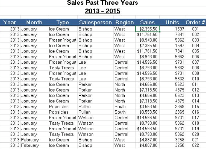
Before creating a pivot table, ensure that your data is properly organized. Ideally, your data should be in a tabular format with column headers and consistent formatting. It’s also helpful to have a clear understanding of the questions you want your pivot table to answer.

Step 2: Select Your Data

Click on any cell within your data range. Then, navigate to the “Insert” tab and click on the “PivotTable” button. Excel will automatically select the range based on your data. Alternatively, you can manually enter the range if Excel doesn’t select it correctly.

Step 3: Customize Your Pivot Table

A new window will appear, prompting you to choose where you want to place your pivot table. Select either a new worksheet or an existing one. Once done, click “OK.”

Step 4: Add Fields to Your Pivot Table

Now it’s time to construct your pivot table. On the right side of the Excel window, you’ll notice a list of column names from your original dataset. Drag and drop these fields into designated sections, such as “Rows,” “Columns,” and “Values.” This arrangement ultimately determines how the data will be summarized and displayed.

Step 5: Apply Filters and Calculations

Excel allows you to filter data within the pivot table by adding fields to the “Filters” section. Additionally, you can perform calculations on the summarized data using functions like SUM, AVERAGE, COUNT, etc. Simply click on any value in the pivot table, select “Value Field Settings,” and apply the desired calculation.

Step 6: Format Your Pivot Table

To make your pivot table visually appealing and easy to read, you can format it. Modify the font, cell color, borders, and other formatting options using the “Design” and “Format” tabs on the Excel ribbon. Experiment with different styles until you achieve the desired look and feel.

Step 7: Refresh Your Pivot Table

If the source data changes, you’ll need to update your pivot table to reflect those changes. Simply right-click on any cell in the pivot table, choose “Refresh,” and Excel will fetch the latest data from the source.

Conclusion

Pivot tables are incredibly valuable for summarizing and analyzing complex data in Excel. By following this step-by-step guide, you can confidently create pivot tables, customize them to fit your needs, apply filters and calculations, format them for visual appeal, and easily refresh the data when necessary. Excel’s pivot table feature empowers you to gain valuable insights from your data, unlocking new possibilities for decision-making and analysis.

Dive into our website and discover the range of Microsoft Office licenses tailored for your database management requirements. With options like an cheap Office 2016 Professional Plus license, a convenient Office 2019 Professional Plus license, and the cheapest Office 2021 Professional Plus license, finding the perfect match has never been easier.