How do I Protect Specific Cells or Ranges in Excel from editing?

Sometimes, you may want to protect certain cells or ranges in your Excel worksheet to prevent accidental changes. In this step-by-step guide, we will show you how to protect specific cells or ranges in Excel.

Step 1: Open Excel and Select the Cells or Ranges

Open your Excel worksheet and select the cells or ranges that you want to protect. You can do this by clicking and dragging the mouse to select the desired cells, or by holding the Ctrl key and clicking on individual cells.

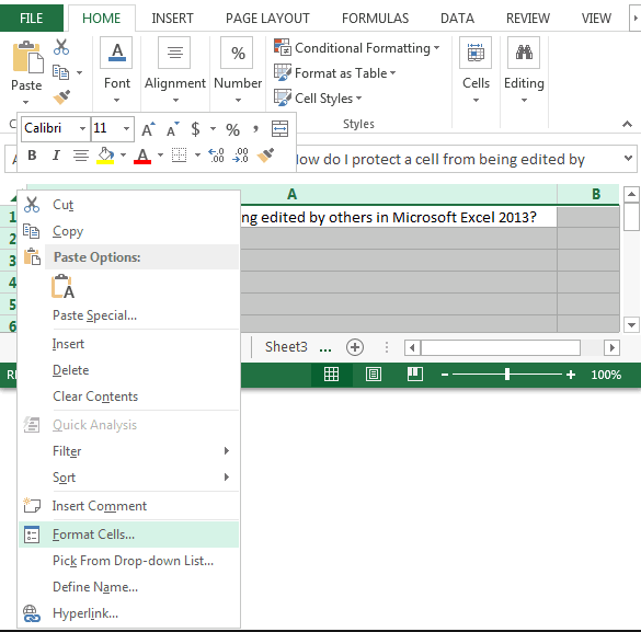
Step 2: Right-click and Choose Format Cells

Once the cells or ranges are selected, right-click on the selection and choose “Format Cells” from the context menu.

Step 3: Go to the Protection Tab

In the Format Cells dialog box, navigate to the “Protection” tab.

Step 4: Check the “Locked” Option

On the Protection tab, check the “Locked” option. This will indicate that the selected cells or ranges will be locked and protected.

Step 5: Protect the Worksheet

To fully protect the selected cells or ranges, you need to protect the worksheet itself. Go to the Review tab in the Excel ribbon, and click on the “Protect Sheet” button.

Step 6: Set Password and Options (Optional)

If you want to set a password to prevent others from unprotecting the sheet, you can do so by entering a password in the “Password to unprotect sheet” field. You can also choose other options, such as allowing some specific users to edit protected cells.

Step 7: Save your Excel Workbook

Save your Excel workbook to preserve the changes and protection settings you have made.

By following these step-by-step instructions, you can easily protect specific cells or ranges in your Excel worksheet, ensuring that important data remains safe from accidental or unauthorized changes.

Unlock incredible savings on Microsoft Office through our website and experience the full potential of this powerful productivity suite.