How can I use the SUMIF and COUNTIF Functions in Excel?

The SUMIF and COUNTIF functions are powerful tools in Excel that allow you to calculate and count data based on specific criteria. In this step-by-step guide, we will show you how to use the SUMIF and COUNTIF functions in Excel.

Step 1: Open Excel and Enter Data

Open Excel and enter the data you want to perform calculations on. For example, enter a list of sales transactions in column A and corresponding sales amounts in column B.

Step 2: Use the SUMIF Function

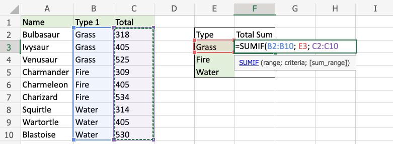
To calculate the sum of values that meet specific criteria, use the SUMIF function. In a new cell, enter the formula =SUMIF(range, criteria, sum_range). For instance, to sum all sales amounts where the product is “Widget“, enter =SUMIF(A:A, "Widget", B:B).

Step 3: Use the COUNTIF Function

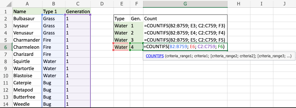
To count the number of cells that match specific criteria, use the COUNTIF function. In a new cell, enter the formula =COUNTIF(range, criteria). For example, to count how many sales transactions were made by a specific salesperson, enter =COUNTIF(A:A, "John").

Step 4: Customize Criteria

You can customize the criteria based on your specific needs. For example, you can use operators like <, >, or <>, or you can use wildcard characters like * or ? to match patterns in your data.

Step 5: Apply Functions to Different Data

To apply SUMIF or COUNTIF functions to different data, simply change the range and criteria in the formulas. The functions will adapt to the new data and perform calculations accordingly.

Step 6: Save your Excel Workbook

Remember to save your Excel workbook to preserve the formulas and data you have entered.

By following these step-by-step instructions, you can effectively use the SUMIF and COUNTIF functions in Excel, enabling accurate calculations and analysis of your data based on specific criteria.

Looking for the best deal on Microsoft Office? Our website offers unbeatable prices to help you tap into the full power of this productivity suite.