
Office Blog
Excel’s Best Chart Types for Business Reports

Microsoft Excel offers a variety of chart types that can help businesses visualize data effectively. Choosing the right chart for your business report is crucial for clear communication and data-driven decision-making. In this guide, we’ll explore the best chart types for different business scenarios and how to use them effectively.
1. Column and Bar Charts – Best for Comparisons
Use When: You need to compare values across categories.
Column and bar charts are among the most commonly used chart types in business reports. They are ideal for comparing performance, revenue, or market trends over time.
Example: Monthly Sales Comparison
If you want to compare sales data for different months:
- Column Chart (Vertical Bars): Best for showing data progression over time.
- Bar Chart (Horizontal Bars): Useful when category names are long.
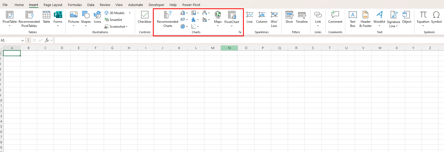
👉 Insert a Column Chart:
- Select your data.
- Go to Insert > Column or Bar Chart and choose your preferred style.
2. Line Charts – Best for Trends and Forecasting
Use When: You need to display trends or track changes over time.
Line charts are ideal for showing fluctuations in data, such as revenue growth, stock prices, or website traffic.
Example: Yearly Revenue Growth
A line chart helps illustrate whether revenue is increasing, decreasing, or stabilizing.
👉 Insert a Line Chart:
- Select your time-based data.
- Go to Insert > Line Chart and select a simple or multi-line option for multiple series.
3. Pie Charts – Best for Showing Proportions
Use When: You need to display percentage distribution.
Pie charts are effective for visualizing how different segments contribute to a whole. They are useful for market share, budget allocation, or customer demographics.
Example: Budget Breakdown
If your business spends 40% on marketing, 30% on operations, and 30% on salaries, a pie chart provides a clear breakdown.
👉 Insert a Pie Chart:
- Select the category and percentage data.
- Go to Insert > Pie Chart and choose a format like 2D, 3D, or Doughnut.
✅ Tip: Avoid using more than 5–6 categories, as too many slices make the chart hard to read.
4. Combo Charts – Best for Comparing Two Data Sets
Use When: You need to compare two different metrics with different scales.
Combo charts combine two types of charts, like a column chart and a line chart, making them ideal for comparing related data sets.
Example: Revenue vs. Profit Margin
If your revenue is in the millions while your profit margin is in percentages, a combo chart helps compare them effectively.
👉 Insert a Combo Chart:
- Select your data.
- Go to Insert > Combo Chart > Custom Combo Chart.
- Choose a column chart for one metric and a line chart for another.
5. Scatter Charts – Best for Identifying Relationships
Use When: You need to visualize correlations between variables.
Scatter charts are excellent for showing patterns or trends between two numerical data sets, like sales and advertising spend.
Example: Sales vs. Marketing Spend
If higher marketing spend results in more sales, a scatter plot will show a clear upward trend.
👉 Insert a Scatter Chart:
- Select two numeric data columns.
- Go to Insert > Scatter Chart and choose a style like straight lines or markers.
6. Waterfall Charts – Best for Financial Reports
Use When: You need to show how values change step-by-step.
Waterfall charts are commonly used in financial reports to illustrate profits, losses, and net balances. They clearly show how each component contributes to a final total.
Example: Profit and Loss Statement
A waterfall chart can break down revenue, expenses, and net income in a clear format.
👉 Insert a Waterfall Chart:
- Select your data.
- Go to Insert > Waterfall Chart.
✅ Tip: Use different colors for positive and negative values to enhance readability.
7. Treemap Charts – Best for Hierarchical Data
Use When: You need to visualize large amounts of categorical data.
Treemap charts display data as nested rectangles, making them great for showcasing market segments, product sales, or expenses.
Example: Product Sales by Category
If your company sells electronics, a treemap can show which products contribute the most revenue.
👉 Insert a Treemap Chart:
- Select your hierarchical data.
- Go to Insert > Treemap Chart.
8. Heatmaps (Conditional Formatting) – Best for Quick Insights
Use When: You need to highlight trends in large datasets.
A heatmap in Excel isn’t a chart but uses Conditional Formatting to apply color coding, making patterns easier to spot.
Example: Sales Performance Across Regions
- High sales can be colored green, and low sales red, making weak areas immediately visible.
👉 Create a Heatmap:
- Select the data range.
- Go to Home > Conditional Formatting > Color Scales.
Choosing the Right Chart for Your Business Report
| Chart Type | Best For |
|---|---|
| Column/Bar Chart | Comparing values across categories |
| Line Chart | Showing trends over time |
| Pie Chart | Displaying percentage breakdowns |
| Combo Chart | Comparing two different data sets |
| Scatter Chart | Identifying correlations |
| Waterfall Chart | Showing financial gains/losses |
| Treemap Chart | Visualizing hierarchical data |
| Heatmaps | Highlighting trends in datasets |
Get the best deals on Microsoft Office keys at unbeatable prices—shop now for the most affordable options!