
Office Blog
Create a PivotTable in Excel in Under 5 Minutes

PivotTable is one of Excel’s most powerful feature, allowing you to summarize and analyze large datasets quickly and effectively. They might seem complex at first, but once you understand the basics, creating a PivotTable is simple and can be done in under five minutes. In this guide, we’ll walk you through the steps to create a PivotTable that will help you quickly analyze your data.
1. What is a PivotTable?
A PivotTable is a tool that allows you to automatically summarize, group, and analyze data. It turns detailed data into an easy-to-read summary, making it easier to find patterns, trends, and insights. With a PivotTable, you can:
- Group data into categories
- Perform calculations like sums, averages, and counts
- Rearrange data quickly to view different perspectives
2. Preparing Your Data
Before creating a PivotTable, make sure your data is organized. Here are some important tips for preparing your data:
- Table Format: Ensure your data is in a table format with columns representing different variables (e.g., Date, Product, Sales).
- No Blank Rows/Columns: Ensure there are no empty rows or columns in your data.
- Headings: Make sure every column has a clear heading (e.g., “Product,” “Sales,” “Region”).
Your data should look something like this:
| Date | Product | Sales | Region |
|---|---|---|---|
| 01/01/2022 | Widget A | 100 | North |
| 01/02/2022 | Widget B | 150 | South |
| 01/03/2022 | Widget A | 120 | North |
| 01/04/2022 | Widget C | 80 | East |
3. Inserting a PivotTable
Now that your data is ready, follow these simple steps to create a PivotTable:
Step 1: Select Your Data
Click anywhere inside your data range. If your data is formatted as a table, you can select any cell within the table. Excel will automatically identify the full range of data.
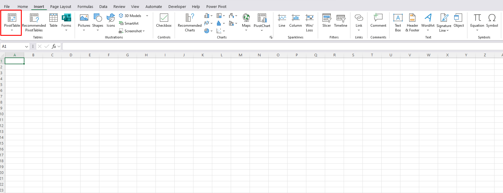
Step 2: Go to the “Insert” Tab
In the Ribbon, click on the Insert tab. You’ll see the “PivotTable” option in the Tables group.
Step 3: Choose PivotTable Location
Click PivotTable, and a dialog box will appear asking you where you want to place the PivotTable. You can choose either:
- New Worksheet: This will create a PivotTable in a new tab.
- Existing Worksheet: This will allow you to place the PivotTable in a location on the same sheet.
Once you’ve selected the location, click OK.
4. Building Your PivotTable
Once you click OK, a blank PivotTable field list will appear. The field list shows the columns from your data and allows you to drag them into different areas to build your PivotTable.
Step 4: Add Fields to Your PivotTable
The key areas of a PivotTable are:
- Rows: Drag fields here to create row labels.
- Columns: Drag fields here to create column labels.
- Values: Drag fields here to perform calculations (sum, average, count, etc.).
- Filters: Drag fields here to filter data in your PivotTable.
Let’s say you want to summarize total sales by product. You would:
- Drag Product to the Rows area.
- Drag Sales to the Values area.
Excel will automatically calculate the sum of sales for each product.
Step 5: Adjust PivotTable Options
- You can right-click on any value in the PivotTable to adjust its settings, like changing the summary function from “Sum” to “Average” or “Count.”
- To add more detail or filter your data, drag additional fields to the Filters or Columns areas.
Get the cheapest Office Keys at unbeatable prices—genuine, fast delivery, and 100% activation guaranteed!