5 Essential Excel Functions Everyone Should Know

Microsoft Excel is a powerful tool for data analysis, financial calculations, and project management, but to get the most out of it, knowing a few essential functions is key. These functions can simplify tasks, help you make data-driven decisions, and save you time. Here are five must-know Excel functions that can elevate your spreadsheet skills.

1. SUM – Quickly Calculate Totals

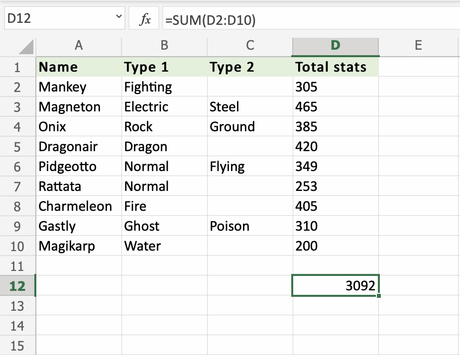
The SUM function is the most basic and widely used Excel function, perfect for adding up numbers in a range of cells.

• Formula: =SUM(range)
• Example: To calculate the total sales in cells A2 to A10, use =SUM(A2:A10).

The SUM function is essential for quickly calculating totals and makes it easy to keep running totals, budget estimates, or project cost calculations. Just select the range you want, and Excel will instantly sum them up.

2. AVERAGE – Calculate Mean Values

The AVERAGE function is useful when you need to find the mean or average of a data set. It’s commonly used for financial analysis, grading, and performance metrics.

• Formula: =AVERAGE(range)
• Example: To find the average sales for a week, use =AVERAGE(A2:A8) if your sales data is in cells A2 to A8.

This function saves you time by automatically calculating the average, which is particularly useful when analyzing large datasets or summarizing performance across categories.

3. IF – Make Decisions in Your Spreadsheet

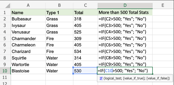
The IF function allows you to perform logical tests and return specific values based on whether the result is true or false. It’s perfect for setting conditions and automating tasks like grading or creating alerts for low inventory.

• Formula: =IF(condition, value_if_true, value_if_false)
• Example: To check if a sales target was met, use =IF(A2 >= 1000, "Target Met", "Below Target").

The IF function makes Excel much more dynamic, allowing for conditional logic. You can use it to set up automated checks, such as flagging overdue payments or classifying performance levels.

4. VLOOKUP – Find Data Across Sheets

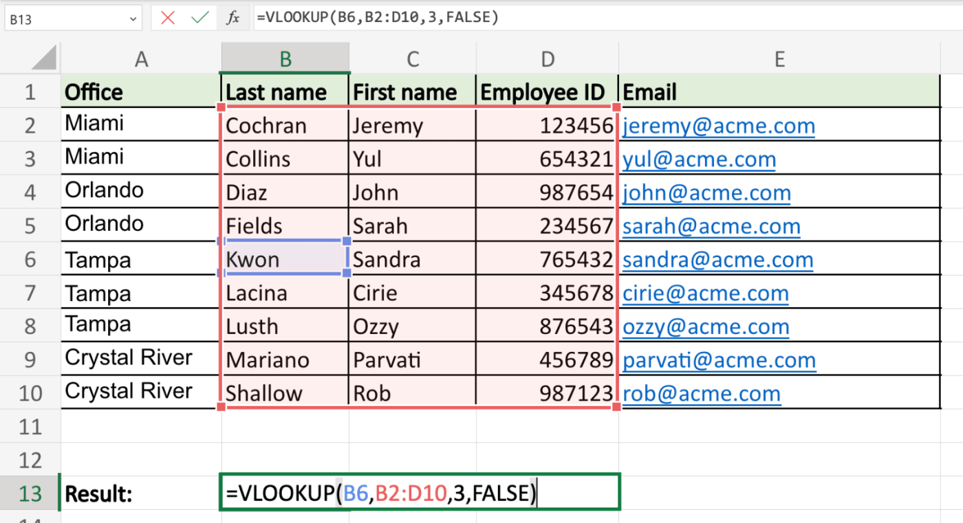
The VLOOKUP (Vertical Lookup) function is essential when you need to find information from different tables or sheets within your workbook. It’s particularly useful for pulling data based on specific criteria, like looking up prices or matching IDs.

• Formula: =VLOOKUP(lookup_value, table_array, col_index_num, [range_lookup])
• Example: To find the price of a product in cell B2 from a list of prices in cells A2, you can use =VLOOKUP(B2, A2:C10, 3, FALSE).

VLOOKUP saves you the hassle of manually searching through large datasets and allows you to retrieve relevant information with ease. However, keep in mind that it works best with structured tables where the lookup values are in the first column.

5. CONCATENATE (or CONCAT) – Combine Text

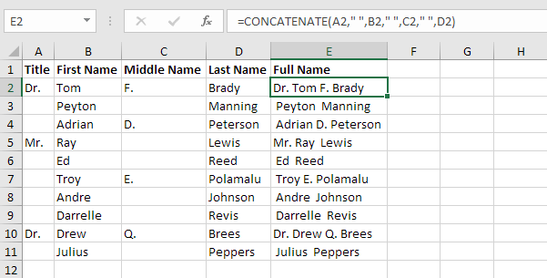
The CONCATENATE (or the newer CONCAT) function is useful for combining text from different cells. This is especially handy for creating labels, generating full names from separate first and last name cells, or formatting addresses.

• Formula: =CONCATENATE(text1, text2, ...) or =CONCAT(cell1, cell2, ...)
• Example: To combine a first name in cell A2 and a last name in cell B2 into one cell, use =CONCATENATE(A2, " ", B2).

CONCATENATE allows for easy customization of text, such as creating custom identifiers or product codes. It’s also great for producing readable labels in reports or organizing data for presentations.

Get genuine Office Keys at an affordable price to unlock the full suite of Microsoft Office tools, boosting productivity for both personal and professional use.